Objectives
Once we've obtained abundance counts for our genes/exons/transcripts, we are usually interested in identifying those genes/exons/transcripts that are differentially expressed.
In this section, you will learn about 4 different tools for identifying differentially expressed genes from gene count data. The same data from the previous exercises will be used. The data contains 75 bp paired-end reads that have been generated in silico to replicate real gene count data from Drosophila. The data simulates two biological groups with three biological replicates per group (6 samples total).
- Learn about DESeq, edgeR, DEXSeq and cuffdiff packages and the differences among these packages.
- Become familiar with basic R usage and installing Bioconductor modules.
- Learn how to use edgeR/DESeq to identify differentially expressed genes.
- Learn how to use cuffdiff pacakge to identify differentially expressed genes.
Get set up
cds

cd my_rnaseq_course
cd gene_expression_exercise
# you should have already copied this over

#modify our gene counts file a bit
grep '^F' gene_counts.htseq.gff > gene_counts.htseq.final.gff
Let's first start installing some R tools because they may take a while.
When following along here, please switch to your idev session for running these example commands.
Introduction
Most RNA-Seq experiments are conducted with the aim of identifying genes/exons that are differentially expressed between two or more conditions. Many computational tools are available for performing the statistical tests required to identify these genes/exons.
Simply put, all these tools do three steps (and they can vary in how they do these steps):
- Normalization of gene counts
- Represent the gene counts by a distribution that defines the relation between mean and variance (dispersion).
- Perform a statistical test on this distribution to identify genes that are significantly different between the conditions.
- Provide fold change, P-value information, false discovery rate for each gene.
Why Normalize?
Normalization smooths out technical variations among the samples we are comparing so that we can more confidently attribute variations we see to biological reasons.
We usually normalize for:
- Sequencing depth: Say we are comparing gene counts in sample A against sample B. If you start out with 10 million reads in sample A vs 1 million reads in sample B, a 10 fold increase in expression in sample A is going to be purely due to its sequencing depth.
- Gene length: A gene that is twice as long is likely to have twice as many reads sampling it.
Most commonly done normalization
RPKM: Normalizes for sequencing depth and gene length.
RPKM = reads per kilobase per million mapped reads
RPK= No.of Mapped reads/ length of transcript in kb (transcript length/1000)
RPKM = RPK/total no.of reads in million (total no of reads/ 1000000)
| DESeq | edgeR | DEXSeq | Cuffdiff | |
|---|---|---|---|---|
| Normalization | Median scaling size factor | Median scaling size factor /TMM | Median scaling size factor | FPKM (a slight variation on RPKM) |
| Distribution | Negative binomial | Negative binomial | Negative binomial | Negative binomial |
| DE Test | Negative binomial test | Fisher exact test | Modified T test | T test |
| Advantages | Straightforward, fast, has a method to work on data with no replicates
| Straightforward, fast, good with small number of replicates. Can handle comparisons across multiple conditions | Good for identifying exon-usage changes | Good for identifying isoform-level changes, splicing changes, promotor changes. Not as straightforward, somewhat of a black box |
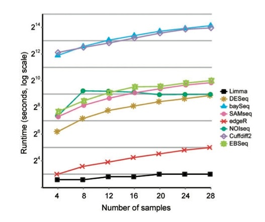
DEG tools compared
From paper: Wesolowski et al, Biosensors, 2013

When following along here, please switch to your idev session for running these example commands.
R and Bioconductor, very briefly...
R is a very common scripting language used in statistics. There are whole courses on using R going on in other SSI classrooms as we speak! Inside the R universe, you have access to an incredibly large number of useful statistical functions (Fisher's exact test, nonlinear least-squares fitting, ANOVA ...). R also has advanced functionality for producing plots and graphs as output.
Regrettably, R is a bit of it's own bizarro world, as far as how its commands work. (Futhermore, Googling "R" to get help can be very frustrating.) The conventions of most other programming and scripting languages seem to have been re-invented by someone who wanted to do everything their own way in R. Just like we write shell scripts in bash, you can write R scripts that carry out complicated analyses.
Do not copy the > characters in the R examples.
They are the R prompt to remind you which commands are to be run inside the R shell!
Hints for working with R
- Don't forget: it's
q()to quit. - For help with a function, type
?command. Try?read.table. Theqkey gets you out of help, just like for amanpage. - The left arrow
<-(less-than-dash) is the same as an equals sign=. You can use them interchangeably. - The prompt we will sometimes be showing for R is
>. Don't type this for a command. It is like thelogin1$at the beginning of the bash prompt when you log in to Lonestar. It just means that you are in theRshell.
You can type the name of a variable to have its value displayed. Like this...
> x <- 10 + 5 + 6
> x
[1] 21
Bioconductor packages for R
Like other languages, R can be expanded by loading packages. The R equivalent of Bioperl or Biopython is Bioconductor. Bioconductor can theoretically do things for you like convert sequences (none of us use it for that), but where it really shines is in doing statistical tests (where is it second-to-none in this list of languages). Many functions for analyzing microarray data are implemented in R, and this strength has now carried over to the analysis of RNAseq data.
Here's how you install two modules that we will need for this exercise: (But first, remember that to get R on lonestar, you'll need to load the R module first)
The install commands may take several minutes to complete. You can read ahead while they run or even open a new terminal window and connect it to Lonestar and continue onward in the tutorial as you wait for R.
login1$ module load R
login1$ R

> source("http://bioconductor.org/biocLite.R")
Warning in install.packages("BiocInstaller", repos = a["BioCsoft", "URL"]) :
  'lib = "/opt/apps/R/2.15.3/lib64/R/library"' is not writable
Would you like to use a personal library instead?  (y/n) y
Would you like to create a personal library
~/R/x86_64-unknown-linux-gnu-library/2.15
to install packages into?  (y/n) y
...
> biocLite("DESeq")
...
> biocLite("edgeR")
...
> q()
Save workspace image? [y/n/c]: n
When you start R later, you will not need to re-install the modules. You can load them with just these commands:
login1$ R
> library("DESeq")
> library("edgeR")
These commands will work for any Bioconductor package!
DESeq
Input:
DESeq takes as input count data in table form, with each column representing a biological replicate/biological condition. The count data must be raw counts of sequencing reads, not already normalized data.
Example:
untreated1 untreated2 untreated3 untreated4 treated1 treated2 treated3
FBgn0000003 0 0 0 0 0 0 1
FBgn0000008 92 161 76 70 140 88 70
FBgn0000014 5 1 0 0 4 0 0
Our gene_counts.htseq.final.gff looks like this, so we can move on to the next steps.
login1$ R
#LOAD LIBRARY, READ IN GENE COUNTS, ADD METADATA
> library("DESeq")
> counts = read.delim("gene_counts.htseq.final.gff", header=F, row.names=1)
> head(counts)
> colnames(counts) = c("C11","C12","C13","C21","C22","C23")
> head(counts)
> my.design <- data.frame(
  row.names = colnames( counts ),
  condition = c( "C1", "C1", "C1", "C2", "C2", "C2"),
  libType = c( "paired-end", "paired-end", "paired-end", "paired-end", "paired-end", "paired-end" )
)
> my.design
> conds <- factor(my.design$condition)


#CREATE A DESEQ DATA OBJECT FROM COUNTS
> cds <- newCountDataSet( counts, conds )
> cds


#NORMALIZATION: ESTIMATE SIZE FACTORS
> cds <- estimateSizeFactors( cds )
> sizeFactors( cds )
> head( counts( cds, normalized=TRUE ) )


#ESTIMATE DISPERSION/VARIANCE
> cds <- estimateDispersions( cds )


#DO TEST FOR DIFFERENTIAL EXPRESSION AND WRITE RESULTS INTO FILE
> result <- nbinomTest( cds, "C1", "C2" )
> head(result)
> result = result[order(result$pval), ]
> head(result)
> write.csv(result, "DESeq-C1-vs-C2.csv")


#GENERATE MA PLOT
> pdf("DESeq-MA-plot.pdf")
> plot(
  result$baseMean,
  result$log2FoldChange,
  log="x", pch=20, cex=.3,
  col = ifelse( result$padj < .1, "red", "black" ) )
> dev.off()
> q()

Save workspace image? [y/n/c]: n
login1$ head DESeq-wt-vs-mut.csv
edgeR
These commands use the negative binomial model, calculate the false discovery rate (FDR ~ adjusted p-value), and make a plot similar to the one from DESeq.
login1$ R

#LOAD LIBRARY, READ IN COUNTS, ADD SOME METADATA
> library("edgeR")
> counts = read.delim("gene_counts.htseq.gff", header=F, row.names=1)
> colnames(counts) = c("C11", "C12", "C13", "C21", "C22", "C23")
> head(counts)
> group <- factor(c("C1", "C1", "C1", "C2", "C2", "C2"))


#CREATE EDGER SPECIFIC DATA OBJECT FROM COUNTS DATA
> dge = DGEList(counts=counts,group=group)


#ESTIMATE DISPERSIONS(VARIANCE)
> dge <- estimateCommonDisp(dge)
> dge <- estimateTagwiseDisp(dge)


#DO TEST FOR DIFFERENTIAL EXPRESSION
> et <- exactTest(dge)
> etp <- topTags(et, n=100000)


#GENERATE MA PLOT
> pdf("edgeR-MA-plot.pdf")
> plot(
  etp$table$logCPM,
  etp$table$logFC,
  xlim=c(-3, 20), ylim=c(-12, 12), pch=20, cex=.3,
  col = ifelse( etp$table$FDR < .1, "red", "black" ) )
> dev.off()


#WRITE OUT GENE RESULTS
> write.csv(etp$table, "edgeR-wt-vs-mut.csv")
> q()
Save workspace image? [y/n/c]: y
login1$ head edgeR-wt-vs-mut.csv
DEXSeq
This package is meant for finding differential exon usage between samples from different conditions.
Relative usage of an exon = transcripts from the gene that contain this exon / all transcripts from the gene
For each exon (or part of an exon) and each sample :
- count how many reads map to this exon
- count how many reads map to other exons of the same gene.
- calculate ratio of 1 to 2.
- Look for changes in this ratio across conditions
- Look for statistically significant changes in this ratio across conditions, by using replicates.
This lets you identify changes in alternative splicing, changes in usage of alternative transcript start sites.

Cuffdiff
Cuffdiff (a part of the tuxedo suite) is a popular tool for testing for differential expression. We will cover this along with the rest of the tuxedo suite tomorrow.
Lets look at our results
head DESeq-wt-vs-mut.csv
head edgeR-wt-vs-mut.csv
- Find the top 10 upregulated genes in both sets
#DESeq results
sed 's/,/\t/g' DESeq-C1-vs-C2.csv|sort -n -r -k6,6|cut -f 2,6|head

#edgeR results
sed 's/,/\t/g' edgeR-wt-vs-mut.csv |sort -n -r -k2,2|cut -f 1,2|head
2. Select DEGs with following cut offs- Fold Change > 2 (this means log 2 fold change > 1) and p value < 0.05 and count how many DEGs we have.
#We will use log 2 fold change instead of fold change because edgeR doesnt report fold change
#DESeq results
sed 's/,/\t/g' DESeq-C1-vs-C2.csv|awk '{if (($7>=1)&&($8<=0.05)) print $1,$7,$8}'|head
sed 's/,/\t/g' DESeq-C1-vs-C2.csv|awk '{if (($7>=1)&&($8<=0.05)) print $1,$7,$8}'|wc -l

#edgeR results
sed 's/,/\t/g' edgeR-wt-vs-mut.csv |awk '{if (($2>=1)&&($3<=0.05)) print $1,$2,$3}'|head
sed 's/,/\t/g' edgeR-wt-vs-mut.csv |awk '{if (($2>=1)&&($3<=0.05)) print $1,$2,$3}'|wc -l
The graphs we generated are located at:
http://web.corral.tacc.utexas.edu/BioITeam/rnaseq_course/DESeq-MA-plot.pdf
http://web.corral.tacc.utexas.edu/BioITeam/rnaseq_course/edgeR-MA-plot.pdf