This tutorial will teach the basics of preprocessing using AFNI. It is helpful to consult this reference either before or after going through this tutorial: https://www.ncbi.nlm.nih.gov/pmc/articles/PMC5102908/. Preprocessing is a bit of a weird name because after "preprocessing" the data are very much processed. (its like saying someone has an undergraduate degree after they graduated). Basically, preprocessing involves cleaning your data for artifacts and noise in order to extract the "True" signal. There are an infinite number of ways that one can preprocess their data. Here are a list of things people typically do to their data and generally how common they are (in my opinion):
- Removing first couple of TRs - very commonly reported
- Despiking (removing outlier spikes in data) - very commonly reported
- Time shifting data to account for differences in acquisition times - very commonly reported
- Volume registration/Alignment to anatomical image - very commonly reported
- Warping to standard space - commonly reported, but not always needed
- Regressing physiological noise, such as heart rate and breathing - Used to be popular, but almost no one does this anymore
- Regressing out non-neuronal brain signal, such as that from white matter or cerebrospinal fluid - commonly reported, but less common recently.
- Regressing out global brain signal (average whole brain signal) - somewhat commonly reported. THIS IS CONTROVERSIAL AND IS NOT USED BY EVERYONE.
- Bandpass filtering 0.01-0.15 Hz signal - this is commonly reported, but is growing out of favor.
- Blurring/Spatial Smoothing - very commonly reported, but not always needed/helpful
- Motion scrubbing (censoring trials with a lot of movement) - very commonly reported and practically required for most papers.
- Removing areas with low signal to noise ratio - not commonly reported, but probably done commonly
In this tutorial, I will demonstrate preprocessing using the bolded steps above. This is how I have gotten accustomed to processing my data, but this habit will likely change when new studies on preprocessing come out. As an example, regressing out white matter and CSF has been found to be useless at best and counter-productive at worst since these areas contain neurogenic signal.
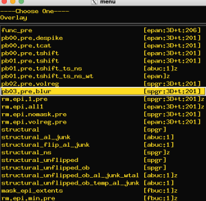
For this tutorial, we will use the "func_pre" and "structural" files. These are "raw" fMRI files, in that they have not been processed yet. However, note that these files don't come out of the scanner this way. Normal scanner files are numerous and need to be constructed into a 3d images. To do this, you will need to consult another tutorial on building scanner images and anatomical processing.
Put both (or all four) of these files into a separate folder called "Preprocessing" (inside your Temp folder; ~/Desktop/Temp/Preprocessing). Let's start preprocessing!
1) Removing the first couple of TRs to eliminate magnetization artifact. When you first begin a scan, the scanner needs time to stabilize its gradients (the things that help create the MR images). This usually takes a second or two. To be safe, a lot of people remove the first couple of TRs. I take out about 5. To remove these, we will use 3dTcat:
3dTcat -prefix pb00.pre.tcat func_pre+orig.'[5..$]' Note the prefix starts with "pb00" and ends with "tcat." The pb stands for "processing block" and tcat is the command we used. This tells us that this was the first processing step we performed (since we are using 0 as 1 in the coding world) and that we used 3dTcat. Let's take a look at our results. Here, what we will do is open two AFNI GUIs. Open two terminals and navigate to the "Preprocessing folder in both," then type afni and hit Enter. Close the visualization windows, but leave one open for each GUI, and separate the afni command windows to either side. Place "func_pre" as the underlay in one afni command window and "pb00.pre.tcat" as the underlay in the other. Now click "Graph" (any direction as long as they are the same) on both of them. Use "jump to xyz" to jump to the same coordinate on both windows. It might not be easy to see the difference between the two graphs, but the pb00 version should be shorter by about 5 TRs. Note that the value for "Num" at the bottom of the graph is different between the two windows. Close both windows when you are satisfied comparing the two files.
2) Despiking. This step helps to reduce the extreme values caused by motion and other factors. Use this command to despike!
3dDespike -NEW -nomask -prefix pb00.pre.despike pb00.pre.tcat+orig. By the naming convention, we are still in processing block "00," but now we have moved on to the "despike" step. Let's compare our despiked and non-despiked images by opening two AFNI GUIs again. Here are the two graph traces from a single voxel across the tcat and despike files:

The figure on the left is non-despiked, and the one on the right is despiked. Note how the values look less extreme (particularly the big spike that touches the bottom of the screen in the left picture).
3) Time shifting data to account for differences in acquisition times. Since fMRI images are acquired sequentially (and not all at once), they will have different acquisition times. Some of the future steps will assume that all the slices were acquired at the same time. So, we have to shift the timing of each slice so that they appear to come at the same TR. For more information on this, see https://andysbrainbook.readthedocs.io/en/latest/fMRI_Short_Course/Preprocessing/Slice_Timing_Correction.html.
3dTshift -tzero 0 -quintic -prefix pb00.pre.tshift pb00.pre.despike+orig. Again, we are in the first processing block, but now we have time-shifted (tshift) our data. We are going to add another step of "deobliquing" our fMRI data. Deobliquing is the process of aligning the image more squarly in native space. Some people's heads will point more towards the corner of the AFNI visualization window. Warping straightens out the person's head so it looks like everyone is looking forward.
3dWarp -deoblique -prefix pb01.pre.tshift pb00.pre.tshift+orig. We have now moved on to processing block 1. Compare the pb00 and pb01 versions of each tshift file through the visualization windows in AFNI. Note that there may not be a big difference if the subject's head is already well aligned.
4) Volume registration/Alignment to anatomical image. One issue with fMRI is that we are taking pictures of the brain while the participant is free to move their heads slightly. This means at every TR, there is a slight change in the position of the voxels relative to the previous TR. To correct for these differences, we use 3dvolreg (volume registration). Basically, we pick a single TR and we align the other images to it. In this case, we are going to take the 3rd TR and perform this function. 3dvolreg is also useful at generating measures of motion from TR to TR. This will be helpful in a future step where we correct for activation changes due to motion. Finally, this function will also create a transformation matrix to align all the images together in a single step. A transformation matrix is basically a map of how to align two images together based on mathematics.
3dvolreg -verbose -zpad 1 -cubic -base pb01.pre.tshift+orig.'[2]' -1Dfile dfile.pre.1D -1Dmatrix_save mat.pre.vr.aff12.1D -prefix rm.epi.volreg.pre pb01.pre.tshift+orig. If you use ls you will notice that there are 3 new files:
mat.pre.vr.aff12.1D - This is the transformation matrix
dfile.pre.1D - Measure of motion between TRs
rm.epi.volreg.pre+orig.BRIK - File with aligned TRs
To see the effect of the alignment, open up AFNI and set pb01.pre.tshift+orig as the underlay. Click "Graph" and hit the "v" button inside the window. In the visualization windows you will see the image of every TR over time. You should notice it bouncing around (up and down, left and right, forward and backwards). Now do the same thing with the rm.epi.volreg.pre+orig. file. You should notice significantly less motion (also if you look at the eyes, you will see them moving from frame to frame). In essence, we have just aligned all the TRs together.
5) Structural/functional alignment. We have just spent some time aligning the TRs together for the functional run, but we also have to align the functional data to the structural data. It is obviously important to do this because without this step, we are not really sure what functional areas we are analyzing. This part of the tutorial has several steps and will take the longest amount of time to process, since it is computationally intense. The first thing we are going to do is to warp our structural image into Talairach (standard) space. Note that we could align the structural and functional images in the subject's native space, but we are not going to do that here.
@auto_tlrc -base TT_N27+tlrc -input structural+orig. If you get an error that the function cannot find the TT_N27 file, try putting it directly in the folder you are working in. After the function is working, you will notice a new file called "structural+tlrc". If you open it in AFNI and set it as the underlay, you will see this file in standard space. Now we can start to align the images. The next step will create a transformation matrix for moving the functional image to standard space. This step takes a good amount of time.
align_epi_anat.py -anat2epi -anat structural+orig. -anat_has_skull no -epi pb01.pre.tshift+orig. -epi_base 2 -epi_strip 3dAutomask -suffix _al_junk -check_flip -volreg off -tshift off -ginormous_move -cost lpc+ZZ. You will notice this step creates a whole bunch of files. The only file that really matters out of all this is structural_al_junk_mat.aff12.1D. This is the transformation matrix that moves the structural image to the functional one. Again, this is like a map that AFNI can use to map out how to move the voxels around to align everything up. So at this point, we have three transformations we made:
- moving the structural image to standarad space with align_epi_anat.py (structural_al_junk_mat.aff12.1D matrix)
- Using 3dvolreg to align the images by TR (mat.pre.vr.aff12.1D)
- Moving the structural image to standard space
Along the way we also created aligned images. However, what we are going to do here is a little unusual. We are going to take all the transformation matrices and information related to alignment and we are going to combine all that together in one single file, and then in one fell swoop, align everything together. Why would we do that when we could just do everything one step at a time like we just did? Well, you get much better alignment results when you combine the transformation steps. So, with that being said, let's combine the movement data together and apply it to create a final aligned data set.
cat_matvec -ONELINE structural+tlrc::WARP_DATA -I structural_al_junk_mat.aff12.1D -I mat.pre.vr.aff12.1D > mat.pre.warp.aff12.1D. Using the function cat_matvec (concatenating matrices and vectors), we created a single roadmap to move our functional data to our structural data, and to align all the images with different TRs. Now, we just have to apply that matrix to the functional data.
3dAllineate -base structural+tlrc -input pb01.pre.tshift+orig -1Dmatrix_apply mat.pre.warp.aff12.1D -mast_dxyz 2 -prefix rm.epi.nomask.pre . Now we should have a fully aligned set of images!!! Open AFNI and put "structural+tlrc" as your underlay and "rm.epi.nomask.pre" as your overlay. The image should look red and yellow.
Checking the alignment is a VERY IMPORTANT step, possibly the most important. So we have to take some time to make sure it looks up to snuff. The way we are going to do this is by removing the overlay so we can make sure the overlay and underlay correspond. Put your cursor over any window and hit "o" repeatedly. You will notice the red and yellow disappearing and reappearing. The question we have to ask ourselves is: Is this alignment good enough? If not, we have a serious problem that requires a whole new tutorial. Either way, we don't want to continue if our alignment is off. Lets make it easier to check the alignment:
- At the upper right part of the AFNI window, you will see the word "OLay" next to the letter "B". Right click on this and hit "Choose colorbar." From here, choose "Spectrum: Red to Blue."

- Next, unclick the "autoRange."
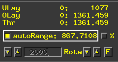
- Here's the tricky part. We are going to mess with the range values so that we get a good contrast between white matter, grey matter, and CSF. Here, I chose a value of about 1200. This is an art more than a science so just choose the values that work for you. You want to be able to identify landmarks on the functional image as well as you can to compare them with the structural image. Let's take a look at some images.


In the above sagittal images, you will notice that the gyri and sulci line up pretty well. Notice the spaces of the sulci on the right and the deeply red colors on the right. They seem to correspond pretty well. You may notice that the reddish color protrudes more superiorly than the structural images does. This is ok. Remember that functional images are measuring properties of blood and there is a lot of blood outside the brain tissue. Let's look at a different set of images:


Here, we want to pay attention to the ventricles (CSF). It looks like the reddish tones match up pretty well with where the ventricles are (and so do the gyri and sulci). The ventricles are a good area to pay attention to because they are an easily identifiable landmark. Keep moving around the brain and looking for good alignment. There will be places where it's not perfect, but it should be as reasonable as shown in the above image. If so, we can move on to other stages of processing.
6) Getting rid of missing data (intro to masks). I haven't mentioned this step up until now, but it's an important one. A "mask" is just a file that identifies specific areas of the brain. They are spatially coded as a non-zero number, where that number indicates a region of interest. In this case, our region of interest happens to be all voxels where data aren't missing. Let's jump through a bunch of commands to make this happen:
3dcalc -overwrite -a pb01.pre.tshift+orig -expr 1 -prefix rm.epi.all1. Makes all voxels in the functional image field of view red (labeled 1).
3dAllineate -base structural+tlrc -input rm.epi.all1+orig -1Dmatrix_apply mat.pre.warp.aff12.1D -mast_dxyz 2 -final NN -quiet -prefix rm.epi.1.pre. Aligns the previous image to everything else in standard space.
3dTstat -min -prefix rm.epi.min.pre rm.epi.1.pre+tlrc. Determines where there is usable data.
3dcopy rm.epi.min.pre+tlrc mask_epi_extents. Copies the file to a different name.
3dcalc -a rm.epi.nomask.pre+tlrc -b mask_epi_extents+tlrc -expr 'a*b' -prefix pb02.pre.volreg. Get rid of any areas with missing data from our functional data set.
If you actually look at the pb02 data file, it doesn't look any different. That's because we don't have much missing data. However, this step is useful if you are missing data in certain areas.
7) Blurring (or "smoothing"). Blurring is very useful at removing certain artifacts and sources of noise (i.e. thermal noise), but can also decrease the ability to localize where signal is coming from in the brain a tad. For a short intro on blurring, go here: https://andysbrainbook.readthedocs.io/en/latest/AFNI/AFNI_Short_Course/AFNI_Preprocessing/05_AFNI_Smoothing.html
3dmerge -1blur_fwhm 4.0 -doall -prefix pb03.pre.blur pb02.pre.volreg+tlrc. Let's take a look at what our data look like after this step. First set your overlay as the pb02 image, and then switch to the pb03 (smoothed) image. Set your underlay to the structural image.By moving up and down in the menu bar, you can compare the two images.
You will notice that, logically, the pb03 is blurrier than the pb02. That was easy!
8) Making a mask of the subjects brain. Just like we made a mask of areas where the subject had data above, we are going to estimate a mask of areas where the subject has brain voxels. Follow these steps:
3dAutomask -dilate 1 -prefix full_mask.pre pb03.pre.blur+tlrc. create 'full_mask' dataset of only brain voxels
3dresample -master full_mask.pre+tlrc -input structural+tlrc -prefix rm.resam.anat. Resample the mask file to the voxel geometry of the functional data set. Note that the structural and functional data sets have different numbers of voxels.
3dmask_tool -dilate_input 5 -5 -fill_holes -input rm.resam.anat+tlrc -prefix mask_anat.pre. Make the mask all 1 values.
9) Scaling. Every person's BOLD activation is different. Some people have subtle shifts in their BOLD signal over time, while others have big fluctuations. In order to perform group level analyses, it's good to have everyone's signal be standardized so that it fluctuates around a certain number and only goes to a certain range. In this case, we are going to make the mean of their signal 100 and their range of values between 0 and 200.
3dTstat -prefix rm.mean_pre pb03.pre.blur+tlrc. Get the mean of the BOLD signal
3dcalc -a pb03.pre.blur+tlrc -b rm.mean_pre+tlrc -c mask_epi_extents+tlrc -expr 'c * min(200, a/b*100)*step(a)*step(b)' -prefix pb04.pre.scale. Scale the signal
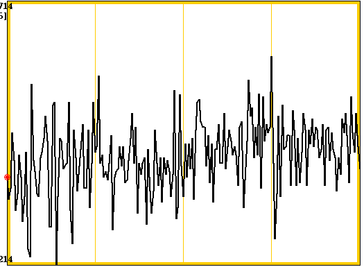
To confirm that it worked, open the pb04.pre.scale file as your underlay and open the "Graph" viewer. Press "v" on the graph to let it move across the TR values. You will notice the "Val" bounce around values near 100.
10) Regression. This one is a doozy, but it's the last step in our preprocessing. Activation and functional connectivity analyses are very corrupted by motion (especially functional connectivity data). So we have to regress out any potential effects of motion. The best way to do this is to identify and remove (i.e. censor) any TRs with a lot of motion. Here, we define "a lot of motion" as an average of 0.3mm per TR in 6 different directions (roll, pitch, yaw, and rotation around each direction). To gather these mathematical data, we will first run a set of commands to setup our regression.
1d_tool.py -infile dfile.pre.1D -set_nruns 1 -demean -write motion_demean.1D. compute de-meaned motion parameters (for use in regression)
1d_tool.py -infile dfile.pre.1D -set_nruns 1 -derivative -demean -write motion_deriv.1D. compute motion parameter derivatives
1d_tool.py -show_mmms -infile motion_deriv.1D > motion_deriv.pre.mmms.txt. compute motion parameter derivatives
1d_tool.py -infile dfile.pre.1D -set_nruns 1 -show_censor_count -censor_prev_TR -censor_motion 0.3 motion. create censor file motion_censor.1D, for censoring motion
1d_tool.py -infile dfile.pre.1D -set_nruns 1 -quick_censor_count 0.3 > TRs_out.pre.txt. create censor file motion_censor.1D, for censoring motion.
1d_tool.py -infile motion_enorm.1D -show_tr_run_counts trs > out.TRs.txt. Count total TRs
IMPORTANT NOTE: At this point this analysis would either be tailored toward looking at task-based activation or resting-state functional connectivity. For simplicity, I am going in the direction of functional connectivity. Task-based activation can be handled in a different tutorial.
Now, we are ready to regress out the effects of head motion. Here is the code:
3dDeconvolve -input pb04.pre.scale+tlrc.HEAD \
-censor motion_censor.1D \
-polort A -float \
-num_stimts 12 \
-stim_file 1 motion_demean.1D'[0]' -stim_base 1 -stim_label 1 roll_01 \
-stim_file 2 motion_demean.1D'[1]' -stim_base 2 -stim_label 2 pitch_01 \
-stim_file 3 motion_demean.1D'[2]' -stim_base 3 -stim_label 3 yaw_01 \
-stim_file 4 motion_demean.1D'[3]' -stim_base 4 -stim_label 4 dS_01 \
-stim_file 5 motion_demean.1D'[4]' -stim_base 5 -stim_label 5 dL_01 \
-stim_file 6 motion_demean.1D'[5]' -stim_base 6 -stim_label 6 dP_01 \
-stim_file 7 motion_deriv.1D'[0]' -stim_base 7 -stim_label 7 roll_02 \
-stim_file 8 motion_deriv.1D'[1]' -stim_base 8 -stim_label 8 pitch_02 \
-stim_file 9 motion_deriv.1D'[2]' -stim_base 9 -stim_label 9 yaw_02 \
-stim_file 10 motion_deriv.1D'[3]' -stim_base 10 -stim_label 10 dS_02 \
-stim_file 11 motion_deriv.1D'[4]' -stim_base 11 -stim_label 11 dL_02 \
-stim_file 12 motion_deriv.1D'[5]' -stim_base 12 -stim_label 12 dP_02 \
-fout -tout -x1D X.xmat.1D -xjpeg X.jpg \
-x1D_uncensored X.nocensor.xmat.1D \
-fitts fitts \
-errts errts \
-x1D_stop \
-bucket stats
This code doesn't actually create a new time series (4D) file, but it creates a file that can be used to regress out the effects of head motion: X.nocensor.xmat.1D. You can view the examples of head motion by typing 1dplot X.nocensor.xmat.1D and hitting Enter on the command line (notice all the wiggles in the top 12 lines):

We can use this file to partially remove the effects of motion in the final two commands:
3dTproject -polort 0 -input pb04.pre.scale+tlrc.HEAD -censor motion_censor.1D -cenmode ZERO -ort X.nocensor.xmat.1D -prefix errts.pre.tproject. detrend model out of data to get error time series
3dcalc -a errts.pre.tproject+tlrc -b full_mask.pre+tlrc -prefix errts.pre -expr 'a*step(b)'. Only include data within the subject's mask (brain voxels).
We have fully preprocessed this person's data! The final file is the "errts.pre" file. Open this up in AFNI as the underlay and check out the graph. It might not seem like anything special, but we can now use this to perform resting-state functional connectivity analyses! Stay tuned!
(If you want to practice this tutorial on your own, try using the "func_post" data set).