This section describes the steps taken analytically and in MATLAB to analyze the kinematic properties of this mechanism alongside some derived mechanical considerations. Note that the beam walking mechanism pulls back the chute as its load but is not rigidly connected to it by joint or other means.
The lazy Susan is a rigid disc like structure where its angular quantities purely depend on the force exerted on its lever to create a torque. It also exists in independence of the beam-walking mechanism.
The approach is to analyze the beam-walking mechanism as a 4 bar mechanism attached in parallel to another 4 bar linkage. This is due to the fact that links 4 and 6 move in parallel to one another and are connected by link 5 which moves purely curvilinearly. Link 7's geometry matches side BP of the ternary link 3 (outlined in green). Link 7's ends are connected to ends B and P by link 5 and 8 respectively at a fixed distance equal to link 8's length.
With this observation in mind, one deduce that all points on link 8 (from end P to the right most point, i.e top of link 7) move in identical fashion with the only change being a horizontal offset in position. These link lengths are optimized to maximize the linear sweep with as least spacing as possible
lengths in mm
- link 1 (O2 to O4, referred to as d) = 148 mm
- link 2 (Crank arm, referred to as a) = 60 mm
- link 3 (AB, coupler, referred to as b) = 123.6 mm
- link 4 ( O4 to B, rocker, referred to as c) = 115 mm
- link 5 (130mm)
- link 6 (identical to link 4) = 115mm
- Identical to length BP = 100.41mm
- link 8, (indentical to link 5) = 130mm
Therefore, by analyzing part of link 1 (the section of ground from O2 to O4), link 2, the line AB from link 3, and link 4, all necessary kinematic information can be retrieved (starting with the use of Gruebler's equation, see 1. Mobility Calculation)
Mobility Calculation (M = 3L - 3 - J1 - J2 )


The figure 3 dimensionally outlines the number of joints in the beam-walking mechanism's links. As shown by the equation below, there is only one degree of freedom, reinforcing the fact the rotation of link 2 manipulates the positions of the connected links.
Vector loop diagram (basis for position, velocity, and acceleration analysis)
Note that there is a switch to a local frame such that the x-axis points in parallel to R1 and y in perpendicular. A conversion to a global frame will be outlined, using the transformation angle γ = 26.5°
Predetermined angular quantities
Ground does not rotate, and given the local frame, θ1 = 0, ω1 = 0, α1 = 0
max rpm of motor to be used at constant 100rpm, thus ω2 = 100 rpm, α2 = 0

Position Analysis find angular quantities (θ3, θ4) and coupler point P's position
1. Position Analysis (nonlinear system of equations solved using a MATLAB algorithm shown later)

2. A use of relative position analysis is utilized. Given the length of link 2, its angular position, the length AB and the ternary angle of the ternary link is 31°, the coupler position can be found

3. Conversion to global frame XY using a rotation matrix

Vector Analysis to find angular quantities (ω3, ω4) (read left to right)
1. Differentiate the vector loop

2. Expand Euler form and create 2 equations from real and imaginary components

3. Design of Machinery's algebraic simplification, followed by definition of point P's velocity.

4. Return to global frame (correction, alpha = 26 is corrected and renamed to γ = 26.5°)

Acceleration Analysis to find angular quantities ( α3, α4)
5. Differentiate velocity equation to obtain acceleration (no coriolis effect to account for)

6. Differentiate velocity equation to obtain acceleration (no coriolis effect to account for). Similarly, by expanding the Euler forms and grouping real and imaginary components for 2 equations, a linear system can be solved.

7. Linear system for angular accelerations after simplification (solved using inversion on MATLAB)

8. Defining the acceleration of Point P in the global frame

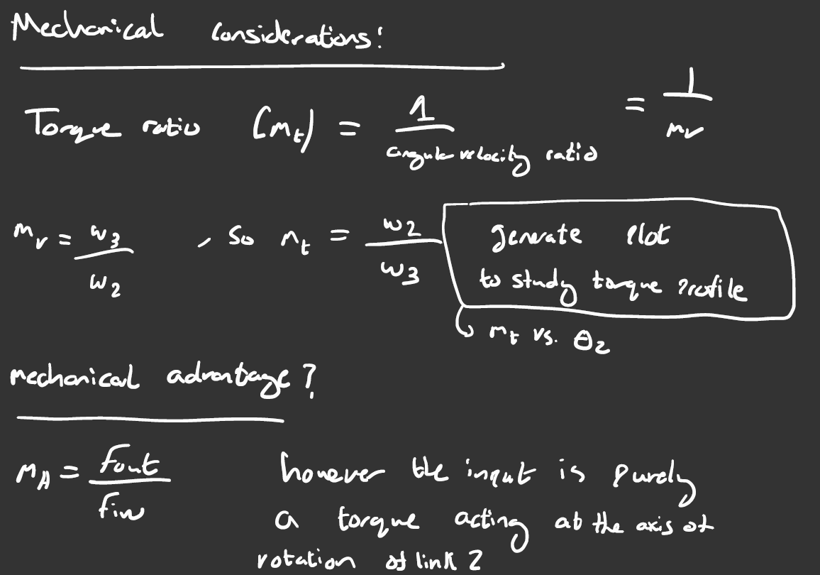
Mechanical Considerations
This subsection aims to use some of the kinematics and motor specifications to quickly extract some mechanical properties about the closed system to provide information about the mechanism's operation
The motor power at its theoretical maximum is the product of the rated voltage and current, which is 13.2W

Generated Plots using MATLAB:

Figure 1: Coupler Point's y-coordinate vs. x-coordinate
Our links deviate from the standard semicircular path but emphasis on extending the linear sweep with as little change in the y-coordinate as possible.

Figure 2: X-velocity & Y-velocity subplots of coupler point vs.θ2

Figure 3: X-acceleration & Y-acceleration subplots of coupler point vs.θ2

Figure 4: Subplots of angular velocity ratio, torque ratio, and outward force on coupler vs. θ2
A thorough observation of the plots shows that the coupler force spikes at roughly 177-180 degrees, which coincides with angular the region where the x position of the coupler is at the leftmost point (pulling the rail fully back) and the region of highest x-acceleration. By the third law of motion, this systematically corresponds to the coupler exerting the highest force on the payload, but extra care must be taken as 200N can damage links, joints, and attachments of small cross sections, especially regions with stress concentration effects.
Solidworks MATLAB generated synthesis and animation:
The animation below shows our walking beam mechanism and the path taken by the pushing arm attached to it, which is our link of interest.
| View file | ||||
|---|---|---|---|---|
|
Beam-Walking mechanism in full range of motion
Code and full kinematic analysis in Appendix.