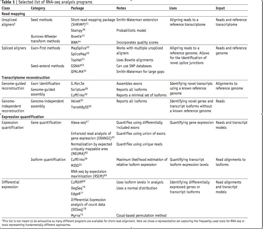
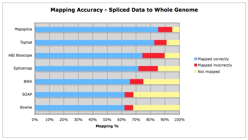
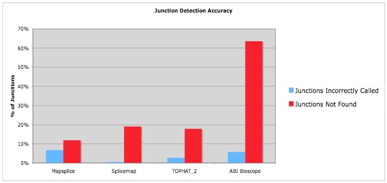
Differential expression with splice variant analysis aug2012

Differential expression with splice variant analysis at the same time: the Tophat/Cufflinks workflow

Some introduction necessary

In this lab, you will explore a fairly typical RNA-seq analysis workflow. Simulated RNA-seq data will be provided to you; the data contains 75 bp paired-end reads that have been generated in silico to replicate real gene count data from Drosophila. The data simulates two biological groups with three biological replicates per group (6 samples total). This simulated data has already been run through a basic RNA-seq analysis workflow. We will look at:

i. How the workflow was run and what steps are involved.
ii. What genes and isoforms are significantly differentially expressed ?

Six raw data files were provided as the starting point: c1_r1, c1_r2, c1_r3 from the first biological group, and c2_r1, c2_r2, and c2_r3 from the second.

Due to the size of the data and length of run time, *most of the programs have already been run for this exercise*. The commands run are in different *.commands files. We will spend some time looking through these commands to understand them. You will then be parsing the output, finding answers, and visualizing results.

mention igenomes: http://tophat.cbcb.umd.edu/igenomes.html

The workflow

The analysis pipeline, graphically:

From: http://dx.doi.org/10.1038/nprot.2012.016

Alternate pipelines

From:

a) map reads against the Drosophila genome (using tophat) (this has already been done to save time)
b) assemble the putative transcripts (using cufflinks) (this has already been done to save time)
c) merge the assemblies (using cuffmerge) (this has already been done to save time)
d) compute differential expression (using cuffdiff) and find genes and isoforms significantly differentially expressed (by parsing output)
e) inspect the results
f) examine the differential expression results (using unix, IGV and cummeRbund)
Extra: g) compare assembled transcripts to annotated transcripts to identify potentially novel ones (using cuffcmp)

You will almost certainly need to consult the documentation for tophat and cufflinks:
http://tophat.cbcb.umd.edu/manual.html
http://cufflinks.cbcb.umd.edu/manual.html

a) and b) Running tophat and cufflinks: Look at tophat.commands and cufflinks.commands to see how tophat and cufflinks were run.

tophat [options] <bowtie_index_prefix> <reads1> <reads2>

cufflinks [options] <hits.bam>

On lonestar, to run tophat, cufflinks etc, following modules need to be loaded.

module load boost/1.45.0
module load bowtie
module load tophat
module load cufflinks/2.0.2

Exercise: If I wanted to provide a trancript annotation file (gtf file) in cufflinks command, what would I add to the command?
i. If I wanted cufflinks to not assemble any novel transcripts outside of what is in the gtf file
ii. If I wanted cufflinks to assemble novel as well as annotated transcripts?

c) Merging assemblies using cuffmerge

find . -name transcripts.gtf > assembly_list.txt
cuffmerge <assembly_list.txt>

d) Finding differentially expressed genes and isoforms using cuffdiff

cuffdiff [options] <merged.gtf> <sample1_rep1.bam,sample1_rep2.bam> <sample2_rep1.bam,sample2_rep2.bam>

Exercise: What does cuffdiff -b do?

e) Inspect the mapped results

Before you even start, do a sanity check on your data by examining the bam files from the mapping output.

I've included the directory "bwa_genome" containing the output from bwa of the C1_R1_1 and C1_R1_2 files mapped directly to the genome using bwa. You might want to load this into IGV alongside the tophat bam file for the same sample to see the differences between mapping to the transcriptome and mapping to the genome (like you lose a bunch of reads).

Report the total number of input reads and the total number of mapped reads for each sample using "samtools flagstat". There is a big difference between the bam file from tophat and the bam file from bwa. Can you spot it? For C1_R1, compare the percentage mapped to the genome to the percentage mapped via tophat/bowtie to the genome.

Now, load ONE of the bam file outputs from the tophat run (remember, tophat calls bowtie for mapping). These are large files; you can load more than one, just be prepared that it may slow your computer down. If you want to load two, I'd suggest loading one from C1 and one from C2 so you see genuine expression level changes.

wget http://www.broadinstitute.org/igv/projects/downloads/IGV_2.1.14.zip
unzip IGV_2.1.14.zip
cd IGV_2.1.14
java -Xmx2g -jar igv.jar

f) Examine the differential expression analysis results

For d), see the file "cuffdiff.sh" and "cuffdiff.sh.log" for the input, command line, and output. Then, find the cuffdiff output (either by understanding cuffdiff.sh or by looking) and by looking at it and/or reading the documentation find the isoforms and genes that are differentially expressed. Note that cuffdiff has performed a statistical test on the expression values between our two biological groups. It reports the FPKM expression levels for each group, the log2(group 1 FPKM/ group 2 FPKM), and a p-value measure of statistical confidence, among many other helpful
data items.

Exercise: Find the number of genes that are differentially expressed at the gene level and the number of genes that are differentially expressed in isoform level. Find the number of genes that are differentially expressed in one (gene/isoform) level, but not in the other. This can be done with a python or perl script, or with a one-line linux command.

cat gene_exp.diff |grep 'yes'|awk '{print $2}'|sort|uniq|wc -l

cat isoform_exp.diff |grep 'yes'|awk '{print $2}'|sort|uniq|wc -l

Here is a basic command useful for parsing/sorting the gene_exp.diff or isoform_exp.diff files:

cat isoform_exp.diff | awk '{print $10 "\t" $4}' | sort -n -r | head

Look at one example of a differentially expressed gene, regucalcin, on IGV.

Using cummeRbund to inspect differential expression data.

module load R
R
>source("http://bioconductor.org/biocLite.R")
>biocLite("cummeRbund")
>library(cummeRbund)
>cuff_data <- readCufflinks('diff_out')

>csScatter(genes(cuff_data), 'C1', 'C2')

>gene_diff_data  <- diffData(genes(cuff_data))
>sig_gene_data  <- subset(gene_diff_data, (significant ==  'yes'))
>nrow(sig_gene_data)


>isoform_diff_data <-diffData(isoforms(cuff_data), 'C1', 'C2')
>sig_isoform_data <- subset(isoform_diff_data, (significant == 'yes'))
>nrow(sig_isoform_data)

>mygene1 <- getGene(cuff_data,'regucalcin')
>expressionBarplot(mygene)
>expressionBarplot(isoforms(mygene))

>mygene2 <- getGene(cuff_data, 'Rala')
>expressionBarplot(mygene2)
>expressionBarplot(isoforms(mygene2))