Objectives
Once we've obtained abundance counts for our genes/exons/transcripts, we are usually interested in identifying those genes/exons/transcripts that are differentially expressed.
In this section, you will learn about different tools for identifying differentially expressed genes from gene count data. The same data from the previous exercises will be used. The data contains 75 bp paired-end reads that have been generated in silico to replicate real gene count data from Drosophila. The data simulates two biological groups with three biological replicates per group (6 samples total).
- Learn about DESeq2, DEXSeq and cuffdiff packages and the differences among these packages.
- Become familiar with basic R usage and installing Bioconductor modules.
- Learn how to use DESeq2 to identify differentially expressed genes.
- Learn how to use cuffdiff pacakge to identify differentially expressed genes.
Introduction
Most RNA-Seq experiments are conducted with the aim of identifying genes/exons that are differentially expressed between two or more conditions. Many computational tools are available for performing the statistical tests required to identify these genes/exons.
Simply put, all these tools do three steps (and they can vary in how they do these steps):
- Normalization of gene counts
- Represent the gene counts by a distribution that defines the relation between mean and variance (dispersion).
- Perform a statistical test for each gene to compare the distributions between conditions.
- Provide fold change, P-value information, false discovery rate for each gene.
Why Normalize?
Normalization smooths out technical variations among the samples we are comparing so that we can more confidently attribute variations we see to biological reasons.
We usually normalize for:
- Sequencing depth: Say we are comparing gene counts in sample A against sample B. If you start out with 10 million reads in sample A vs 1 million reads in sample B, a 10 fold increase in expression in sample A is going to be purely due to its sequencing depth.
- Gene length: A gene that is twice as long is likely to have twice as many reads sampling it.
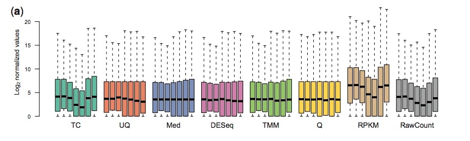
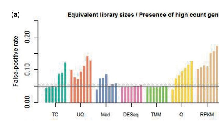
From: Dillies A et al, A comprehensive evaluation of normalization methods for Illumina high-throughput RNA sequencing data analysis,
onsdoi:10.1093/bib/bbs046 .
Most commonly done normalization
RPKM: Normalizes for sequencing depth and gene length.
RPKM = reads per kilobase per million mapped reads
RPK= No.of Mapped reads/ length of transcript in kb (transcript length/1000)
RPKM = RPK/total no.of reads in million (total no of reads/ 1000000)
| DESeq2 | edgeR | DEXSeq | Ballgown | |
|---|---|---|---|---|
| Normalization | Median scaling size factor | TMM | Median scaling size factor | FPKM , but also has provisions for others |
| Distribution | Negative binomial | Negative binomial | Negative binomial | Negative binomial |
| DE Test | Negative binomial test | Fisher exact test | Modified T test | T test |
| Advantages | Straightforward, fast, DESeq2 allows for complicated study designs, with multiple factors | Straightforward, fast, good with small number of replicates. | Good for identifying exon-usage changes | Good for identifying isoform-level changes, splicing changes, promotor changes. Not as straightforward, somewhat of a black box |
Get set up
cds

cd my_rnaseq_course
cd day_3_partA/gene_expression_exercise
# you should have already copied this over
Let's first start installing some R tools because they may take a while.
When following along here, please switch to your idev session for running these commands.
R and Bioconductor, very briefly...
R is a very common scripting language used in statistics. There are whole courses on using R going on in other SSI classrooms as we speak! Inside the R universe, you have access to an incredibly large number of useful statistical functions (Fisher's exact test, nonlinear least-squares fitting, ANOVA ...). R also has advanced functionality for producing plots and graphs as output.
Regrettably, R is a bit of it's own bizarro world, as far as how its commands work. (Futhermore, Googling "R" to get help can be very frustrating.) The conventions of most other programming and scripting languages seem to have been re-invented by someone who wanted to do everything their own way in R. Just like we write shell scripts in bash, you can write R scripts that carry out complicated analyses.
module spider Rstats

module load intel/18.0.2
module load Rstats/4.0.3
Hints for working with R
- Don't forget: it's
q()to quit. - For help with a function, type
?command. Try?read.table. Theqkey gets you out of help, just like for amanpage. - The left arrow
<-(less-than-dash) is the same as an equals sign=. You can use them interchangeably. - The prompt we will sometimes be showing for R is
>. Don't type this for a command. It is like thelogin1$at the beginning of the bash prompt when you log in to stampede. It just means that you are in theRshell.
You can type the name of a variable to have its value displayed. Like this...
R

#Where are you in R- this is your working directory
getwd()

#Change working directory
setwd(mydirectory)

 x <- 10 + 5 + 6
 x
[1] 21

#Vectors- single data type
id <- c(1,2,3,4,5)
sex<- c("male","male","female","female","female")
id
sex

#Lists-multiple data types
x<-list(1:3, c("Dave", "Van", "Lesa"), c("male","male","female"))
x
str(x)
#Factors- predefined categorial variables
vfact <- factor(sex)
vfact

#Data frames - most tables get read into as data frames-lots of equal length vectors.
mydata <- data.frame(id,sex)
mydata
names(mydata) <- c("Person's ID","Person's sex")
mydata
#Functions to look at data structures
length(id)
typeof(id)
str(x)
summary(mydata)
class(mydata)
names(mydata)

#Reading data from files
read.table()
?read.table()
#Writing data into files
write.table()

#To see all the objects we have available
ls()

#to save all your objects and your command history within R
save.image(file="test.Rdata")
savehistory(file="test.Rhistory")

#when you reenter R, load already created objects and commands
load(file="test.Rdata")
loadhistory(file = "test.Rhistory")

#to quit out of R
q()

#to run a R script from the command line
R CMD BATCH <rscript>
Bioconductor packages for R
R modules on TACC are a little strange. Many of the required packages are available as part of biocontainers, but they don't play well with each other because they are built and load different versions of R. So, I've found a workaround for this by loading one of the R packages we need as a biocontainer module (DESeq2), but installing the other helper packages locally (using a newer version of R).
Like other languages, R can be expanded by loading packages. The R equivalent of Bioperl or Biopython is Bioconductor. Bioconductor can theoretically do things for you like convert sequences (none of us use it for that), but where it really shines is in doing statistical tests (where is it second-to-none in this list of languages). Many functions for analyzing microarray data are implemented in R, and this strength has now carried over to the analysis of RNAseq data.
Here's how you install one package that we will need for this exercise: (But first, remember that to get R on stampede2, you'll need to load the R module or have a version of R installed locally)
Use IDEV Session
The install commands may take several minutes to complete.
!!Make sure to do this in the IDEV session!!
#These commands will work for any Bioconductor package!

R
#should be R.4.0.3 since that is the version of the R module we loaded

#within R
	if (!requireNamespace("BiocManager", quietly = TRUE))
    install.packages("BiocManager")

BiocManager::install("tximport") #we need this pacakge for easily reading in kallisto output for differential expression analysis using DESeq2
#It will ask you if you want to install this in your personal R library. Please say yes.
q()
#You can say no to saving workspace for this step
If it works successfully, you will see a Done('tximport') message. When you start R later, you will not need to re-install the modules. You can load them with library('txpimport') command.
Now, we will load the DESeq2 module that is part of biocontainers. This will load an older version of R along with it, so from now on, when you open R, by default, it will be older than R 4.0.3.
module load biocontainers
module load r-empiricalfdr.deseq2/ctr-1.0.3--r3.3.2_0
DESeq2 Input:
DESeq2 takes as input count data in several forms: a table form, with each column representing a biological replicate/biological condition. DESEQ2 can also read data directly from htseq results, so we can use the 6 files we generated using htseq as input for DESeq2. The count data must be raw counts of sequencing reads, not already normalized data.
Example:
C1_R1 C1_R2 C1_R3 C2_R1 C2_R2 C2_R2
FBgn0000003 0 0 0 0 0 0
FBgn0000008 92 161 76 70 140 88
FBgn0000014 5 1 0 0 4 0
DESeq2 (with the use of an additional packages called tximport and readr) can read data directly from kallisto abundance files. We will need to provide the location of the 6 abundance files, the sample names associated to each file and a Sample Table that gives the mapping between sample and condtion.
SampleName Condition
DESeq2 Scripts:
- DESeq2 script to work with kallisto count output is provided below.
R

#load libraries
library(tximport)
library("DESeq2")


#Import a file called file_list with all the locations of the abundance.tsv files
#eg below:
#/stor/SCRATCH/sample1/abundances.tsv
#/stor/SCRATCH/sample2/abundances.tsv
#/stor/SCRATCH/sample3/abundances.tsv
#/stor/SCRATCH/sample4/abundances.tsv
files<-as.character(read.table("file_list", header=FALSE)$V1)
#Import a file called samples with the sample names corresponding to each file in the file_list
#eg below:
#sample1
#sample2
#sample3
#sample4
#look at the data structures
files

samples<-as.character(read.table("samples",header=FALSE)$V1)
names(files)<-samples
#look at the data structures
samples
files

#Import a file called sampletable which is a tab-delimited file that contains each samplename along with the condition
#eg below:
#samples        condition
#sample1        alc
#sample2        alc
#sample3        con
#sample4        con
sampleTable <-read.table("sampleTable",header=TRUE, row.names=1)
#look at the data structure
head(sampleTable)


#IMPORTANT: MAKE SURE THE SAMPLES AND FILE_LIST ARE IN THE SAME ORDER- SAMPLES SHOULD MATCH UP WITH FILES
samples==rownames(sampleTable) #should return TRUE for all


#Import a file called tx2gene.csv which a csv file that contains the transcript id to gene id mapping
#For Drosophila, this is located at: tx2gene.csv
tx2gene <- read.csv("tx2gene.csv")
#look at this data structure
#read in kallisto abundance files, summarizing by gene
txi <- tximport(files, type = "kallisto", tx2gene = tx2gene)
names(txi)


#make a deseq2 object from the kallisto summarized counts
ddsMatrix <- DESeqDataSetFromTximport(txi, sampleTable, ~condition)
ddsMatrix


#Optionally, if you want to save this count matrix as a file
write.csv(assay(ddsMatrix), file="genecounts.raw.csv", quote=FALSE)

#Optionally, if you want to save normalized counts matrix as a file
ddsMatrix<- estimateSizeFactors(ddsMatrix)
normalized_counts <- counts(ddsMatrix, normalized=TRUE)
write.csv(normalized_counts, file="genecounts.normalized.csv", quote=FALSE)

#Optionally, if you want to do variance stabilizing transformation or regularized log transformation on this count matrix and then save as a file: This can become input to things like wgcna, pca
vsd<- vst(ddsMatrix, blind=TRUE)
write.csv(assay(vsd), file="genecounts.variancestabilized.csv", quote=FALSE)

#estimate size factors, dispersion, normalize and perform negative binomial test to compare across conditions
dds<-DESeq(ddsMatrix)
#collect results from the statistical testing, order by adjusted pvalue and write into an output file
res<-results(dds)
resOrdered <- res[order(res$padj),]
summary(res)
write.csv(resOrdered, "deseq2_kallisto_C1_vs_C2.csv")

#generate MA plot
pdf('MAPlot.pdf')
plotMA(dds,ylim=c(-2,2),main="DESeq2")
dev.off()


#save the R data and history
save.image(file="deseq2.kallisto.Rdata")
savehistory(file="deseq2.kallisto.Rhistory")
R CMD BATCH deseq2.kallisto.R
2. DESeq2 script to work with Htseq count output
library("DESeq2")

#GET HTSEQ COUNTS AND SET UP SAMPLE TABLE
directory<-(getwd())
samples <- c("C1_count1.gff", "C1_count2.gff", "C1_count3.gff", "C2_count4.gff", "C2_count5.gff", "C2_count6.gff")
conditions <- c("control", "control", "control", "treated","treated","treated")
sampleTable<-data.frame(sampleName=samples, fileName=samples, condition=conditions)
sampleTable


#BUILD A DESEQ2 OBJECT FROM THE HTSEQ COUNTS DATA
ddsHTSeq<-DESeqDataSetFromHTSeqCount(sampleTable=sampleTable, directory=directory, design=~condition)
colData(ddsHTSeq)$condition<-factor(colData(ddsHTSeq)$condition, levels=c("control", "treated"))


#LOOK AT THE DESEQ2 OBJECT WE'VE CREATED BY READING IN HTSEQ COUNT FILES
ddsHTSeq

Optionally, if you want to save this count matrix as a file
write.csv(assay(ddsHTSeq), file="genecounts.raw.csv", quote=FALSE)

#Optionally, if you want to save normalized counts matrix as a file
ddsHTSeq<- estimateSizeFactors(ddsHTSeq)
normalized_counts <- counts(ddsHTSeq, normalized=TRUE)
write.csv(normalized_counts, file="genecounts.normalized.csv", quote=FALSE)

#Optionally, if you want to do variance stabilizing transformation or regularized log transformation on this count matrix and then save as a file: This can become input to things like wgcna, pca
vsd<- vst(ddsHTSeq)
write.csv(assay(vsd), file="genecounts.variancestabilized.csv")

#RUN THE STATISTICAL TEST IN ONE GO- NORMALIZATION, ESTIMATE DISPERSION/VARIANCE AND DO TEST FOR DIFFERENTIAL EXPRESSION
dds<-DESeq(ddsHTSeq)
res<-results(dds)
res<-res[order(res$padj),]
mcols(res,use.names=TRUE)
summary(res)

#GENERATE MA PLOT
png('MAPlot_htseq.png')
plotMA(dds,ylim=c(-2,2),main="DESeq2")
dev.off()

#WRITE RESULTS INTO FILE
write.csv(as.data.frame(res),file="deseq2_htseq_C1_vs_C2.csv")
#IF YOU DIDNT WANT TO RUN THE SCRIPT INTERACTIVELY
R CMD BATCH deseq2.htseq.R
If you have counts table *(not from htseq or Kallisto), here's a deseq2 script you could use deseq2.counts.R
DESeq2 Output:
DESeq2 output is a tab-delimited file with the following columns:
GeneName baseMean log2FoldChange lfcSE stat pvalue padj
1.GeneName: Name of feature (gene/transcript)
2.BaseMean: Mean expression of that gene across all samples
3.log2FoldChange: Log2 (ratio of expression in condition1/expression in condition2)
4.lfcSE: Standard error for log fold change
5.stat: Test statistic (t-statistic, for example)
6.pvale: Pvalue- the probability of seeing as extreme or more extreme of a test statistic if the null hypothesis were true
7.padj: Pvaule adjusted for multiple testing error (typically benjamini hochberg corrected Pvalue)
head results/deseq2_kallisto_C1_vs_C2.csv
Find the top 10 upregulated genes
#DESeq2 results
sed 's/,/\t/g' results/deseq2_kallisto_C1_vs_C2.csv|sort -n -r -k3,3|cut -f 1,3|head


#Notice the idiosyncracy with sort
sed 's/,/\t/g' results/deseq2_kallisto_C1_vs_C2.csv|sort -n -r -k3,3|grep -v 'e-0'|cut -f 1,3|head
Find the top 10 downregulated genes
#DESeq2 results

sed 's/,/\t/g' results/deseq2_kallisto_C1_vs_C2.csv|sort -n -k3,3|cut -f 1,3|head

#Notice the idiosyncracy with sort
sed 's/,/\t/g' results/deseq2_kallisto_C1_vs_C2.csv|sort -n -k3,3|grep -v 'e-0'|cut -f 1,3|head
2. Select DEGs with following cut offs- Fold Change >=2 (or <= -2) (this means log 2 fold change >= 1 or <=-1) and adj p value < 0.05 and count how many DEGs we have
#DESeq2 results
sed 's/,/\t/g' results/deseq2_kallisto_C1_vs_C2.csv|awk '{if ((($3>=1)||($3<=-1))&&($7<=0.05)) print $1,$3,$7}'|wc -l
If you wanted to use DESeq2 for more complicated designs (with multiple factors, multiple levels), you can by adjusting two things: design and contrast.
Advanced options
#One factorddsHTSeq<-DESeqDataSetFromHTSeqCount(sampleTable=sampleTable, directory=directory, design=~condition)#Two factors (one factor has multiple levels): condition (control, treated), and sequencing type (single, paired, matepair)ddsHTSeq<-DESeqDataSetFromHTSeqCount(sampleTable=sampleTable, directory=directory, design=~type + condition)#Fold changes will by default be provided for condition (treated vs control)res <- results(dds)#To view fold changes for sequencing type, use contrastres <- results(dds, contrast = c("type", "paired", "single"))res <- results(dds, contrast = c("type", "matepair", "single")) |
DEXSeq
This package is meant for finding differential exon usage between samples from different conditions.
Relative usage of an exon = transcripts from the gene that contain this exon / all transcripts from the gene
For each exon (or part of an exon) and each sample :
- count how many reads map to this exon
- count how many reads map to other exons of the same gene.
- calculate ratio of 1 to 2.
- Look for changes in this ratio across conditions
- Look for statistically significantchanges in this ratio across conditions, by using replicates.
This lets you identify changes in alternative splicing, changes in usage of alternative transcript start sites.

Ballgown
Ballgown (a part of the new tuxedo suite) is a popular tool for testing for differential expression. We will cover this along with the rest of the tuxedo suite.
BACK TO COURSE OUTLINE