Overview
In this lab, we'll look at how to use cummeRbund to visualize our gene expression results from cuffdiff. CummeRbund is part of the tuxedo pipeline and it is an R package that is capable of plotting the results generated by cuffdiff.

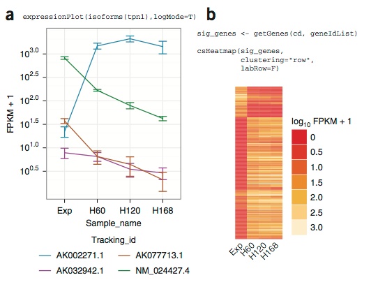
Figure from: Differential gene and transcript expression analysis of RNA-seq experiments with TopHat and Cufflinks, Trapnell et al, Nature Protocols, 2013.
Introduction
CummeRbund is powerful package with many different functions. Cuffdiff produces a lot of output files and all the output files are related by sets by IDs.
#If you have a local copy:
ls -l cuffdiff_results

-rwxr-x--- 1 daras G-801020  2691192 Aug 21 12:20 isoform_exp.diff  : Differential expression testing for transcripts
-rwxr-x--- 1 daras G-801020  1483520 Aug 21 12:20 gene_exp.diff     : Differential expression testing for genes
-rwxr-x--- 1 daras G-801020  1729831 Aug 21 12:20 tss_group_exp.diff: Differential expression testing for primary transcripts
-rwxr-x--- 1 daras G-801020  1369451 Aug 21 12:20 cds_exp.diff      : Differential expression testing for coding sequences

-rwxr-x--- 1 daras G-801020  3277177 Aug 21 12:20 isoforms.fpkm_tracking
-rwxr-x--- 1 daras G-801020  1628659 Aug 21 12:20 genes.fpkm_tracking
-rwxr-x--- 1 daras G-801020  1885773 Aug 21 12:20 tss_groups.fpkm_tracking
-rwxr-x--- 1 daras G-801020  1477492 Aug 21 12:20 cds.fpkm_tracking

-rwxr-x--- 1 daras G-801020  1349574 Aug 21 12:20 splicing.diff  : Differential splicing tests
-rwxr-x--- 1 daras G-801020  1158560 Aug 21 12:20 promoters.diff : Differential promoter usage
-rwxr-x--- 1 daras G-801020   919690 Aug 21 12:20 cds.diff       : Differential coding output
CummeRbund makes managing and querying this data easier by loading the data into multiple objects of several different classes and having functions to query them. Because all of this gets stored in an sql database, you can access it quickly without loading everything in to memory.
- readCufflinks- Most important function designed to read all the output files that cuffdiff generates into an R data object (of class CuffSet).
- cuff_data <- readCufflinks(diff_out)

- CummeRbund has at least 6 classes that it will place different parts of your data in.
- Now you can access information using different functions: gene information using genes(cuff_data), your isoform level output using isoforms(cuff_data), TSS related groups using tss(cuff_data) and so forth
What can you do with cummeRbund?
- Global statistics on data for quality, dispersion, distribution of gene expression scores etc.

- Plot things for specific features or genes
- Data exploration- This are more advanced steps. You can look at your data in a genome browser like view, do PCA, do clustering etc. It claims to be able to even do GO analysis.

Figures from http://compbio.mit.edu/cummeRbund/manual_2_0.html
Get your data
MAKE SURE YOU ARE IN THE IDEV SESSION FOR THIS!
cds
cd my_rnaseq_course
cp -r /corral-repl/utexas/BioITeam/rnaseq_course/diff_results .
cd diff_results


#We need the cuffdiff results because that is the input to cummeRbund.
A) First load R and enter R environment
#module load R will not work for this R package because its needs the latest version of R. So, we'll load a local version.
$BI/bin/R


What is $BI here?
B) Within R environment, install package cummeRbund
source("http://bioconductor.org/biocLite.R")
biocLite("cummeRbund")
C) Load cummeRbund library and read in the differential expression results. If you save and exit the R environment and return, these commands must be executed again.
library(cummeRbund)
cuff_data <- readCufflinks('cuffdiff_results')
D) Use cummeRbund to visualize the differential expression results.
NOTE: Any graphic outputs will be automatically saved as "Rplots.pdf" which can create problems when you want to create multiple plots with different names in the same process. To save different plots with different names, preface any of the commands below with the command:
pdf(file="myPlotName.pdf")
And after executing the necessary commands, add the line:
dev.off()
Exercise 1: Generate a scatterplot comparing genes across conditions C1 vs C2.
pdf(file="scatterplot.pdf")

csScatter(genes(cuff_data), 'C1', 'C2')

dev.off()


#How does this plot look? What is it telling us?
The resultant plot is here.
Exercise 2a: Pull out from your data, significantly differentially expressed genes and isoforms.
#Below command is equivalent to looking at the gene_exp.diff file that we spent a lot of time parsing yesterday
gene_diff_data <- diffData(genes(cuff_data))
#Do gene_diff_data followed by tab to see all the variables in this data object

sig_gene_data  <- subset(gene_diff_data, (significant ==  'yes'))

#Count how many we have
nrow(sig_gene_data)

#Below command is equivalent to looking at the isoform_exp.diff file

isoform_diff_data <-diffData(isoforms(cuff_data))
sig_isoform_data <- subset(isoform_diff_data, (significant == 'yes'))

#Count how many we have
nrow(sig_isoform_data)


Why do we have so many? Yesterday we saw a lot less.
Exercise 2b: Pull out from your data, genes that are significantly differentially expressed and above log2 fold change of 1
#Below command is equivalent to looking at the gene_exp.diff file that we spent a lot of time parsing yesterday
gene_diff_data <- diffData(genes(cuff_data))
#Do gene_diff_data followed by tab to see all the variables in this data object

sig_gene_data  <- subset(gene_diff_data, (significant ==  'yes'))
up_gene_data  <- subset(sig_gene_data, (log2_fold_change > 1))
#How many
nrow(up_gene_data)

#Pause here to consider a mistake I made yesterday


down_gene_data <- subset(sig_gene_data, (log2_fold_change < -1))
nrow(up_gene_data)
Exercise 3: For a gene, regucalcin, plot gene and isoform level expression.
pdf(file="regucalcin.pdf")
mygene1 <- getGene(cuff_data,'regucalcin')
expressionBarplot(mygene1)
expressionBarplot(isoforms(mygene1))
dev.off()
The resultant plot is here.
Exercise 4: For a gene, Rala, plot gene and isoform level expression.
pdf(file="rala.pdf")
mygene2 <- getGene(cuff_data, 'Rala')
expressionBarplot(mygene2)
expressionBarplot(isoforms(mygene2))
dev.off()
Take cummeRbund for a spin...
CummeRbund is powerful package with many different functions. Above was an illustration of a few of them. Try any of the suggested exercises below to further explore the differential expression results with different cummeRbund functions.
If you would rather just look at the resulting graphs, the links to each of the resultant graphs is given below the commands.
You can refer to the cummeRbund manual for more help and remember that ?functionName will provide syntax information for different functions.
http://compbio.mit.edu/cummeRbund/manual.html
Exercise 5: Visualize the distribution of fpkm values across the two different conditions using a boxplot.
The resultant graph is here.
The resultant plot is here.
Exercise 6: Visualize the significant vs non-significant genes using a volcano plot.
The resultant plot is here.
Exercise 7: MORE COMPLICATED! Generate a heatmap for genes that are upregulated and significant.
The resultant plot is here.