...
Figure 1: Overview of WGCNA package

Download sample data files and R code here: WGCNA.zip onto your desktop
Explanation of sample dataset: Time series of coral larval development from 4 hours post fertilization (Day 0) to 245 hours post fertilization (Day 12). Multiple other quantitative traits were measured through the time series. Only green and red fluorescence are added as quantitative traits in the sample dataset. Dataset has 48 samples total, four replicates (A-D) over 12 days. The goal is to find genes that correlate with developmental traits through time and differences in gene expression between early larval development and late larval development.
Step 1: upload data into R and reformat for WGCNA
| Code Block | ||
|---|---|---|
| ||
# Only run the following commands once to install WGCNA and flashClust on your computer
source("http://bioconductor.org/biocLite.R")
biocLite("WGCNA")
install.packages("flashClust")


# Load WGCNA and flashClust libraries every time you open R
library(WGCNA)
library(flashClust)


#Set your current working directory (where all your files are)
setwd("~/Desktop/WGCNA/") # Change the text within quotes as necessary. I have downloaded and unzipped the WGCNA folder on my Desktop


# Uploading data into R and formatting it for WGCNA --------------
# This creates an object called "datExpr" that contains the normalized counts file output from DESeq2
datExpr = read.csv("SampleTimeSeriesRLD.csv")
# "head" the file to preview it
head(datExpr) # You see that genes are listed in a column named "X" and samples are in columns


# Manipulate file so it matches the format WGCNA needs
row.names(datExpr) = datExpr$X
datExpr$X = NULL
datExpr = as.data.frame(t(datExpr)) # now samples are rows and genes are columns
dim(datExpr) # 48 samples and 1000 genes (you will have many more genes in reality)


# Run this to check if there are gene outliers
gsg = goodSamplesGenes(datExpr, verbose = 3)
gsg$allOK


#If the last statement returns TRUE, all genes have passed the cuts. If not, we remove the offending genes and samples from the data with the following:
#if (!gsg$allOK)
#	{if (sum(!gsg$goodGenes)>0)
#		printFlush(paste("Removing genes:", paste(names(datExpr)[!gsg$goodGenes], collapse= ", ")));
#		if (sum(!gsg$goodSamples)>0)
#			printFlush(paste("Removing samples:", paste(rownames(datExpr)[!gsg$goodSamples], collapse=", ")))
#		datExpr= datExpr[gsg$goodSamples, gsg$goodGenes]
#		}


#Create an object called "datTraits" that contains your trait data
datTraits = read.csv("Traits_23May2015.csv")
head(datTraits)
#form a data frame analogous to expression data that will hold the clinical traits.
rownames(datTraits) = datTraits$Sample
datTraits$Sample = NULL
table(rownames(datTraits)==rownames(datExpr)) #should return TRUE if datasets align correctly, otherwise your names are out of order


# You have finished uploading and formatting expression and trait data
# Expression data is in datExpr, corresponding traits are datTraits


save(datExpr, datTraits, file="SamplesAndTraits.RData")
#load("SamplesAndTraits.RData")

# Cluster samples by expression ----------------------------------------------------------------
A = adjacency(t(datExpr),type="signed") # this calculates the whole network connectivity
k = as.numeric(apply(A,2,sum))-1 # standardized connectivity
Z.k = scale(k)
thresholdZ.k = -2.5 # often -2.5
outlierColor = ifelse(Z.k<thresholdZ.k,"red","black")
sampleTree = flashClust(as.dist(1-A), method = "average")


# Convert traits to a color representation where red indicates high values
traitColors = data.frame(numbers2colors(datTraits,signed=FALSE))
dimnames(traitColors)[[2]] = paste(names(datTraits))
datColors = data.frame(outlier = outlierColor,traitColors)
plotDendroAndColors(sampleTree,groupLabels=names(datColors),
                    colors=datColors,main="Sample Dendrogram and Trait Heatmap")


# Day "0" outliers have been identified. You could exclude these samples with the code below, but this scientists had a biological reason to NOT exclude these samples. It's up to you. Justify whatever decision you make.


#Remove outlying samples
#remove.samples = Z.k<thresholdZ.k | is.na(Z.k)
#datExprOut = datExpr[!remove.samples,]
#datTraitsOut = datTraits[!remove.samples,]
#save(datExprOut, datTraitsOut, file="SamplesAndTraits_OutliersRemoved.RData")
|
Figure 2: Clustering of samples and traits. Day 0-12 are categorical traits (1 or 0). Hour post fertilization (HPF), RedFluoro, and Green Fluoro are quantitative traits measured for each sample.
| View file | ||||
|---|---|---|---|---|
|
At this point you will need to identify sample outliers and choose a soft threshold power. These are easy to do and are well documented in the online tutorials. Scripts for choosing a soft threshold are in the attached R file. It's important to choose the correct soft threshold for your dataset.
...
Lecture: WGCNA Concepts
R script: WGCNAshortTutorial.R
Get set up for the exercise:
| Warning |
|---|
When following along here, please switch to your idev session for running these example commands. |
If you have not requested an idev session, do so now:
| Code Block | ||
|---|---|---|
| ||
ssh <username>@stampede2.tacc.utexas.edu

idev -m 120 -q normal -A UT-2015-05-18 -r RNASeq-Thu |
| Code Block | ||
|---|---|---|
| ||
 #We will be doing all this in the idev session
 cds
cd my_rnaseq_course/day_4_partA/wgcna |
Explanation of sample dataset: Time series of coral larval development from 4 hours post fertilization (Day 0) to 245 hours post fertilization (Day 12). Multiple other quantitative traits were measured through the time series. Only green and red fluorescence are added as quantitative traits in the sample dataset. Dataset has 48 samples total, four replicates (A-D) over 12 days. The goal is to find genes that correlate with developmental traits through time and differences in gene expression between early larval development and late larval development.
The complete R script has been provided for you, so you run it using R CMD BATCH. Or you can open up an R prompt and run key pieces of it by copy-pasting bits of code from below. This is to understand what the code is actually doing.
TRAIT DATA FILE: Traits_23May2015.csv
| Code Block | ||
|---|---|---|
| ||
module load intel/18.0.2
module load Rstats/4.0.3 |
| Code Block | ||
|---|---|---|
| ||
module load biocontainers
module load r-flashclust/ctr-1.01_2--r3.3.2_0
module load r-wgcna/ctr-1.51--r3.3.2_0 |
| Code Block | ||
|---|---|---|
| ||
R CMD BATCH WGCNAshortTutorial.R |
Below are the details of the R code you just kicked off above. NO NEED TO RUN THESE LINE BY LINE!
Step 1: upload data into R and reformat for WGCNA (This is all run under the R console)
| Code Block | ||
|---|---|---|
| ||
# Only run the following commands once to install flashClust if needed
#install.packages("flashClust")


# Load WGCNA and flashClust libraries every time you open R
library(WGCNA)
library(flashClust)


# Uploading data into R and formatting it for WGCNA
# This creates an object called "datExpr" that contains the normalized counts file output from DESeq2
datExpr = read.csv("SampleTimeSeriesRLD.csv")
# "head" the file to preview it
head(datExpr) # You see that genes are listed in a column named "X" and samples are in columns


# Manipulate file so it matches the format WGCNA needs
row.names(datExpr) = datExpr$X
datExpr$X = NULL
datExpr = as.data.frame(t(datExpr)) # now samples are rows and genes are columns
dim(datExpr) # 48 samples and 1000 genes (you will have many more genes in reality)


# Run this to check if there are gene outliers
gsg = goodSamplesGenes(datExpr, verbose = 3)
gsg$allOK


#If the last statement returns TRUE, all genes have passed the cuts. If not, we remove the offending genes and samples from the data with the following:
#if (!gsg$allOK)
#	{if (sum(!gsg$goodGenes)>0)
#		printFlush(paste("Removing genes:", paste(names(datExpr)[!gsg$goodGenes], collapse= ", ")));
#		if (sum(!gsg$goodSamples)>0)
#			printFlush(paste("Removing samples:", paste(rownames(datExpr)[!gsg$goodSamples], collapse=", ")))
#		datExpr= datExpr[gsg$goodSamples, gsg$goodGenes]
#		}


#Create an object called "datTraits" that contains your trait data
datTraits = read.csv("Traits_23May2015.csv")
head(datTraits)
#form a data frame analogous to expression data that will hold the clinical traits.
rownames(datTraits) = datTraits$Sample
datTraits$Sample = NULL
table(rownames(datTraits)==rownames(datExpr)) #should return TRUE if datasets align correctly, otherwise your names are out of order
head(datTraits)


# You have finished uploading and formatting expression and trait data
# Expression data is in datExpr, corresponding traits are datTraits


save(datExpr, datTraits, file="SamplesAndTraits.RData")
#load("SamplesAndTraits.RData")
|
At this point you will need to identify sample outliers and choose a soft threshold power. These are easy to do and are well documented in the online tutorials. It is suggested that you cluster samples by expression to identify any outliers before this step. This is provided in the attached R script.
| Code Block | ||
|---|---|---|
| ||
# Choose a soft threshold power- USE A SUPERCOMPUTER IRL ------------------------------------

powers = c(c(1:10), seq(from =10, to=30, by=1)) #choosing a set of soft-thresholding powers
sft = pickSoftThreshold(datExpr, powerVector=powers, verbose =5, networkType="signed") #call network topology analysis function

sizeGrWindow(9,5)
par(mfrow= c(1,2))
cex1=0.9
plot(sft$fitIndices[,1], -sign(sft$fitIndices[,3])*sft$fitIndices[,2], xlab= "Soft Threshold (power)", ylab="Scale Free Topology Model Fit, signed R^2", type= "n", main= paste("Scale independence"))
text(sft$fitIndices[,1], -sign(sft$fitIndices[,3])*sft$fitIndices[,2], labels=powers, cex=cex1, col="red")
abline(h=0.90, col="red")
plot(sft$fitIndices[,1], sft$fitIndices[,5], xlab= "Soft Threshold (power)", ylab="Mean Connectivity", type="n", main = paste("Mean connectivity"))
text(sft$fitIndices[,1], sft$fitIndices[,5], labels=powers, cex=cex1, col="red")

#from this plot, we would choose a power of 18 becuase it's the lowest power for which the scale free topology index reaches 0.90 |
Figure 2: Soft Thresholding: from this plot, we would choose a power of 18 since it's the lowest power for which the scale free topology index reaches 0.90 (red line)
| View file | ||||
|---|---|---|---|---|
|

Step 2: Construct a gene co-expression network and identify modules
| Code Block | ||
|---|---|---|
| ||
#build a adjacency "correlation" matrix enableWGCNAThreads() softPower = 18 adjacency = adjacency(datExpr, power = softPower, type = "signed") #specify network type head(adjacency) # Construct Networks- USE A SUPERCOMPUTER IRL ----------------------------- #translate the adjacency into topological overlap matrix and calculate the corresponding dissimilarity: TOM = TOMsimilarity(adjacency, TOMType="signed") # specify network type dissTOM = 1-TOM # Generate Modules -------------------------------------------------------- # Generate a clustered gene tree geneTree = flashClust(as.dist(dissTOM), method="average") plot(geneTree, xlab="", sub="", main= "Gene Clustering on TOM-based dissimilarity", labels= FALSE, hang=0.04) #This sets the minimum number of genes to cluster into a module minModuleSize = 30 dynamicMods = cutreeDynamic(dendro= geneTree, distM= dissTOM, deepSplit=2, pamRespectsDendro= FALSE, minClusterSize = minModuleSize) dynamicColors= labels2colors(dynamicMods) MEList= moduleEigengenes(datExpr, colors= dynamicColors,softPower = 18softPower) MEs= MEList$eigengenes MEDiss= 1-cor(MEs) METree= flashClust(as.dist(MEDiss), method= "average") save(dynamicMods, MEList, MEs, MEDiss, METree, file= "Network_allSamples_signed_RLDfiltered.RData") #plots tree showing how the eigengenes cluster together the eigengenes cluster together #INCLUE THE NEXT LINE TO SAVE TO FILE #pdf(file="clusterwithoutmodulecolors.pdf") plot(METree, main= "Clustering of module eigengenes", xlab= "", sub= "") #set a threhold for merging modules. In this example we are not merging so MEDissThres=0.0 MEDissThres = 0.0 merge = mergeCloseModules(datExpr, dynamicColors, cutHeight= MEDissThres, verbose =3) mergedColors = merge$colors mergedMEs = merge$newMEs #INCLUE THE NEXT LINE TO SAVE TO FILE #dev.off() #plot dendrogram with module colors below it #plot dendrogram with module colors below it #INCLUE THE NEXT LINE TO SAVE TO FILE #pdf(file="cluster.pdf") plotDendroAndColors(geneTree, cbind(dynamicColors, mergedColors), c("Dynamic Tree Cut", "Merged dynamic"), dendroLabels= FALSE, hang=0.03, addGuide= TRUE, guideHang=0.05) moduleColors = mergedColors colorOrder = c("grey", standardColors(50)) moduleLabels = match(moduleColors, colorOrder)-1 MEs = mergedMEs #INCLUE THE NEXT LINE TO SAVE TO FILE #dev.off() save(MEs, moduleLabels, moduleColors, geneTree, file= "Network_allSamples_signed_nomerge_RLDfiltered.RData") |
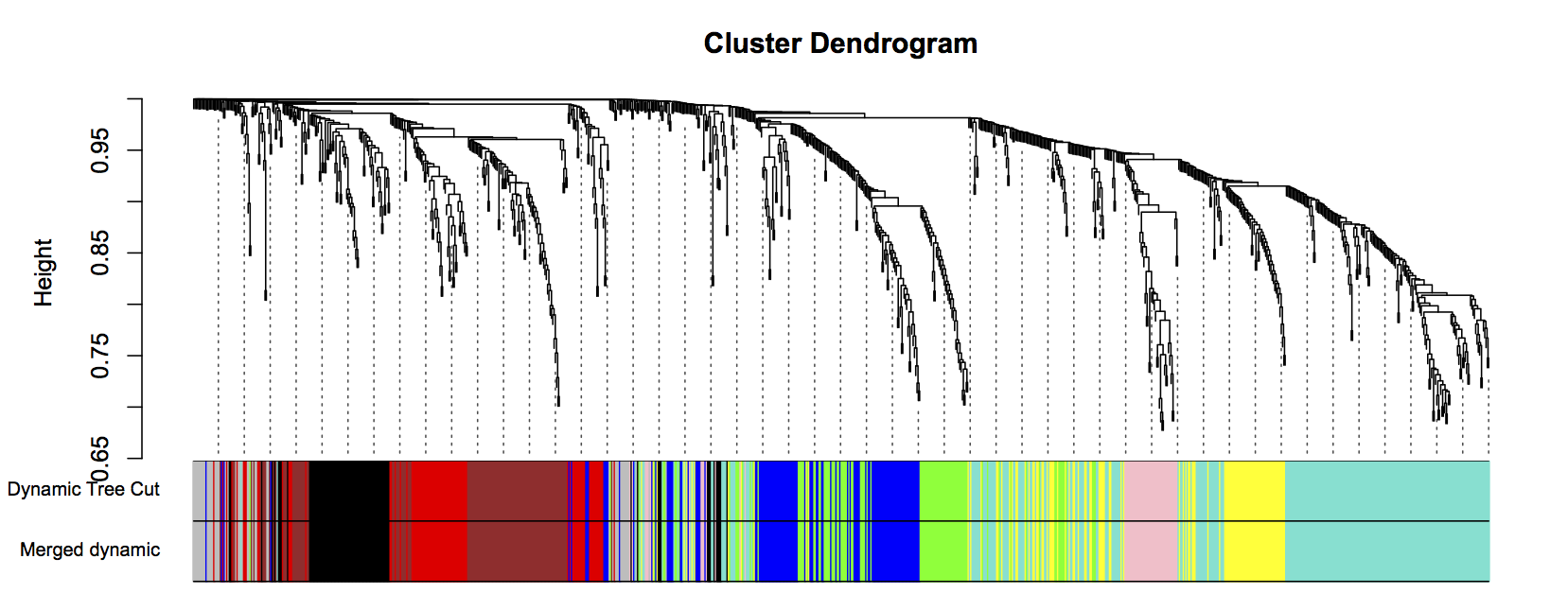
Figure 43: Clustering dendrogram of all genes, with dissimilarities based on topological overlap. Each vertical line represents a single gene. Assigned module colors below.
| View file | ||||
|---|---|---|---|---|
|
.
Step 3: Relate modules to external traits
| Code Block | ||
|---|---|---|
| ||
# Correlate traits --------------------------------------------------------


#Define number of genes and samples
nGenes = ncol(datExpr)
nSamples = nrow(datExpr)
#Recalculate MEs with color labels
MEs0 = moduleEigengenes(datExpr, moduleColors)$eigengenes
MEs = orderMEs(MEs0)
moduleTraitCor = cor(MEs, datTraits, use= "p")
moduleTraitPvalue = corPvalueStudent(moduleTraitCor, nSamples)


#Print correlation heatmap between modules and traits
textMatrix= paste(signif(moduleTraitCor, 2), "\n(",
						signif(moduleTraitPvalue, 1), ")", sep= "")
dim(textMatrix)= dim(moduleTraitCor)
par(mar= c(6, 8.5, 3, 3))


#display the corelation values with a heatmap plot
#INCLUE THE NEXT LINE TO SAVE TO FILE
#pdf(file="heatmap.pdf")
labeledHeatmap(Matrix= moduleTraitCor,
			xLabels= names(datTraits),
			yLabels= names(MEs),
			ySymbols= names(MEs),
			colorLabels= FALSE,
			colors= blueWhiteRed(50),
			textMatrix= textMatrix,
			setStdMargins= FALSE,
			cex.text= 0.5,
			zlim= c(-1,1),
			main= paste("Module-trait relationships"))
#INCLUE THE NEXT LINE TO SAVE TO FILE
#dev.off() |
Figure 54: Module-Trait relationships. Color scale (red-blue) represents the strength of the correlation between the module and the trait. For example, the turquoise module is highly significantly correlated with HPF, RedFluoro and GreenFluoro. Each box gives a correlation value (R^2) followed by p-value (in parenthesis).
| View file | ||||
|---|---|---|---|---|
|
...

For further analysis, if you wanted to pull out genes belonging to a certain module, you can use the following command: