...
| Code Block | ||
|---|---|---|
| ||
 #We will be doing all this in the idev session
 cds
 cd my_rnaseq_data/day_4_partA/wgcna
 module load Rstats
 module load RstatsPackages
R |
Explanation of sample dataset: Time series of coral larval development from 4 hours post fertilization (Day 0) to 245 hours post fertilization (Day 12). Multiple other quantitative traits were measured through the time series. Only green and red fluorescence are added as quantitative traits in the sample dataset. Dataset has 48 samples total, four replicates (A-D) over 12 days. The goal is to find genes that correlate with developmental traits through time and differences in gene expression between early larval development and late larval development.
...
| Code Block | ||
|---|---|---|
| ||
# Choose a soft threshold power- USE A SUPERCOMPUTER IRL ------------------------------------

powers = c(c(1:10), seq(from =10, to=30, by=1)) #choosing a set of soft-thresholding powers
sft = pickSoftThreshold(datExpr, powerVector=powers, verbose =5, networkType="signed") #call network topology analysis function

sizeGrWindow(9,5)
par(mfrow= c(1,2))
cex1=0.9
plot(sft$fitIndices[,1], -sign(sft$fitIndices[,3])*sft$fitIndices[,2], xlab= "Soft Threshold (power)", ylab="Scale Free Topology Model Fit, signed R^2", type= "n", main= paste("Scale independence"))
text(sft$fitIndices[,1], -sign(sft$fitIndices[,3])*sft$fitIndices[,2], labels=powers, cex=cex1, col="red")
abline(h=0.90, col="red")
plot(sft$fitIndices[,1], sft$fitIndices[,5], xlab= "Soft Threshold (power)", ylab="Mean Connectivity", type="n", main = paste("Mean connectivity"))
text(sft$fitIndices[,1], sft$fitIndices[,5], labels=powers, cex=cex1, col="red")

#from this plot, we would choose a power of 18 becuase it's the lowest power for which the scale free topology index reaches 0.90 |
Figure 2: Soft Thresholding: from this plot, we would choose a power of 18 since it's the lowest power for which the scale free topology index reaches 0.90 (red line)
...
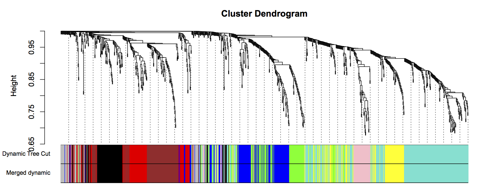
Figure 3: Clustering dendrogram of all genes, with dissimilarities based on topological overlap. Each vertical line represents a single gene. Assigned module colors below.
Step 3: Relate modules to external traits
...
...